This is a follow-up from a previous post in which I discussed how multi-layer perceptrons learn non-linear transformations that embed the input data into a new space in which the classes are linearly separable. The visualisations in that post can give you a clear picture of how the transformation works once the hidden layer perceptrons have already been trained, but what does the output layer see while training is still ongoing, and how does that affect the training process itself?
The other day I was playing around with a neural network implementation comparing my results with the scikit-learn MLPClassifier implementation to get a sense for which tricks and optimisations are most effective. I plotted training accuracy at each epoch to monitor my network’s progress as it trained. If you’ve ever trained a neural network you’ve probably used such a plot. They typically look something like this:
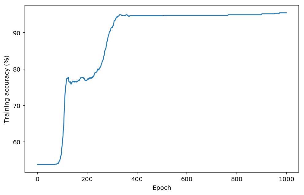
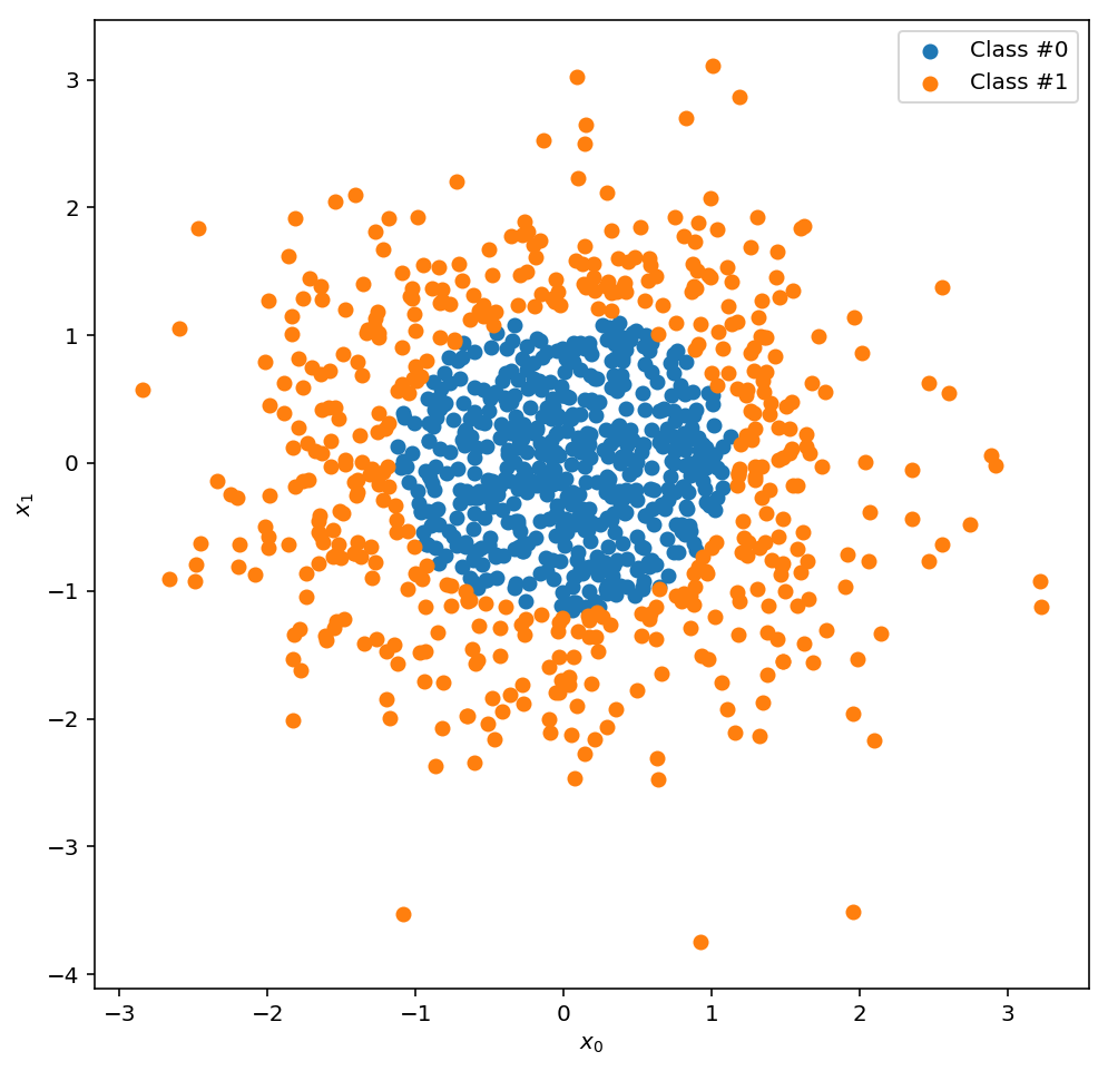
One key feature of these plots that shows up again and again is the cliff and plateau pattern: as the network trains it spends a lot of time making very little progress, and then all of a sudden it finds some new trick and the accuracy shoots up to a new higher plateau. So I began to wonder: what is going on in these plateaus? And is there anything I can do to “fast-forward” through them to the good bits, the cliffs, where the network seems to learn rapidly? To explore these questions, I’ve made a visualisation of the hidden layer outputs after each training epoch. In this classification problem, the initial dataset is two dimensional, and has two classes, one containing everything close to the origin (class 0) and another containing everything else (class 1):
The network I’m training has a hidden layer with 3 nodes, and an output layer with 1 node that classifies the data as 0 or 1. Below there are two plots. On the left is a visualisation of what the output node “sees” as input after a given epoch, which are the outputs of the 3 hidden layer nodes. Blue points are class 0 and red points are class 1. On the right is a plot of the training accuracy at each epoch, with a marker to indicate the training accuracy for the chosen epoch. Try moving the epoch slider to see how the hidden layer transformation changes as the network learns.
Recall that the function of the output node is to find a decision boundary (in this case a 2D plane) through this space that cleanly separates the data into the two classes. So if the red and blue points are all jumbled together, the output node will not be able to find a separating plane and the training accuracy will be low. Conversely, if the red and blue points are spread out and clustered among their own class, the output node should be able find a good decision boundary and the training accuracy will be high.
In the beginning, at epoch 0, the network has been randomly initialised with small weights taken from the normal distribution, so the hidden layer outputs are all clustered around the origin. The training accuracy plateaus until around epoch 140, at which point it shoots up significantly. However, looking at the hidden layer outputs during epochs 0 to 140, a lot of changes have been happening! The network first spread the data up along the z-axis, then rotated it to fall along a line in the x-y plane, and then finally discovered a new feature that shot a new strand of data up the z-axis. Just as it discovers this new feature, the training accuracy starts to ramp up significantly. And you can see why: around epoch 150 the blue points are mostly around the origin and the red points are scattered up the z-axis and into the x-y plane. You could imagine drawing a plane that shears off the corner of the plot where the origin is, so that red points are mostly above the plane and blue points are mostly below, trapped between it and the origin.
There is another training accuracy plateau from around epoch 160 to 280 in which the accuracy wiggles between 0.75 and 0.78. Again, this apparent steadiness belies some interesting changes that are happening in the hidden layer. The transformed data is being spread along all three axes now, pushing the red points out away from the origin but leaving the blue points close to it. At epoch 280 the results of this change start to appear in the training accuracy, and it shoots up again to stabilise around 0.95. The same decision boundary plane from before, cutting out the corner around the origin, works even better now. The training accuracy enters a final plateau, and the hidden layer continues to spread the data in the same directions. Perhaps if I trained the network long enough it would find a new way to transform the data to get the final 5% that it is failing to classify.
So what have we seen? Is there any way to fast-forward through the accuracy plateaus to speed up training? Unfortunately, no: when the training accuracy isn’t moving, the network is doing work that will be the foundation for the next rapid rise in accuracy. If we had found that in those plateaus the network is stuck in a rut, flailing around randomly and retrying the same missteps over and over, then perhaps we could help it along by introducing more randomness to “jump start” it, or by offering some guidance, e.g. by eliminating parts of the search space, or introducing new features or heuristics. But in this case, there is not much we can do.
This phenomena highlights the danger of placing too much emphasis on training accuracy when assessing the progress of the network. During any one of those plateaus, you might have started to believe that the network wasn’t working and decided to cut training short. If the network was actually making progress, you’d have mistakenly wasted all the training that had already gone into it. On the other hand, if the network really was stuck in a rut, continuing training would also be a waste of time. Is there a better metric that we can use to monitor our network as it learns?
Mean squared error is a good candidate: instead of just checking whether the network classified correctly or not, it accounts for how far off the prediction was. This is much more similar to the actual maximum likelihood error function that the network is minimising through gradient descent, but has the advantage of being cheap to compute at each epoch. Thus, the improvements that the network makes during those training accuracy plateaus are discernible in the mean-squared error, as you can see here:
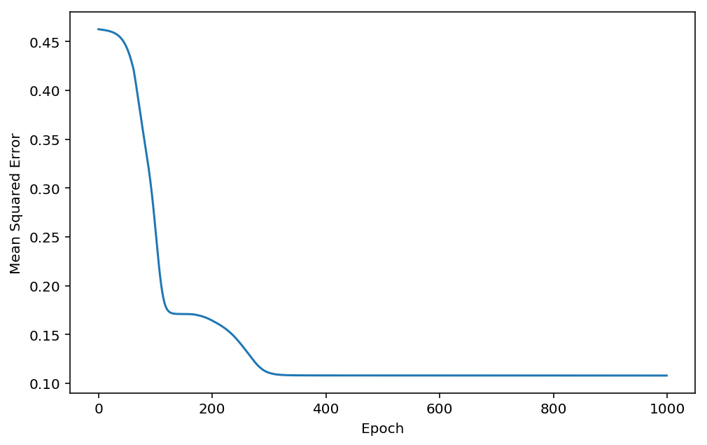
Therefore, and perhaps surprisingly, the mean squared error is a better choice for measuring training progress, even when the final metric you’re interested in is training accuracy.
Below I’ve provided my neural network implementation so that you can try this out for yourself. It’s a simple network with a single hidden layer, and it uses ReLU activations and sigmoid activation gradients. Most importantly, it keeps a history of all the weights it has learned and the accuracy and mean squared error at each epoch, so that you can play back the training process. Enjoy!
import numpy as np
import time
import sys

def sigmoid(X):
    return 1. / (1. + np.exp(-X))

def sigmoid_grad(X):
    return sigmoid(X) * ( 1 - sigmoid(X) )

def relu(X):
    return (X + np.abs(X)) / 2.

def relu_grad(X):
    return sigmoid(X)

class NeuralNetworkWithHistory(object):
    def __init__(self, num_input=2, num_hidden=2, num_output=1, learning_rate=0.1, num_epochs=10, activation='relu'):
        self.num_input = num_input
        self.num_hidden = num_hidden
        self.num_output = num_output
        self.learning_rate = learning_rate
        self.num_epochs = num_epochs

        self.weights_0_1 = np.zeros((num_input, num_hidden))
        self.weights_1_2 = np.random.randn(num_hidden, num_output)

        self.activation, self.activation_grad = self._activation_function(activation)
        self.training_accuracy = np.zeros((self.num_epochs))
        self.mse = np.zeros((self.num_epochs))
        self.weights_0_1_history = np.zeros((self.num_epochs, num_input, num_hidden))
        self.weights_1_2_history = np.zeros((self.num_epochs, num_hidden, num_output))

    def _activation_function(self, name):
        funcs = {
            'relu': (relu, relu_grad),
            'sigmoid': (sigmoid, sigmoid_grad),
        }
        return funcs[name]

    def _forward(self, X):
        self.input = X
        self.hidden = self.activation(np.dot(self.input, self.weights_0_1))
        self.output = self.activation(np.dot(self.hidden, self.weights_1_2))
        return self.output

    def fit(self, X, y):
        n = X.shape[0]
        start = time.time()
        num_progress_bars = 20

        for i in range(self.num_epochs):
            self._forward(X)
            error = y - self.output
            self.grad_output = error * self.activation_grad(self.output)
            self.grad_hidden = np.dot(self.grad_output, self.weights_1_2.T) * self.activation_grad(self.hidden)
            self.dw_1_2 = np.dot(self.hidden.T, self.grad_output)
            self.dw_0_1 = np.dot(self.input.T, self.grad_hidden)
            self.weights_1_2 += self.learning_rate * self.dw_1_2 / n
            self.weights_0_1 += self.learning_rate * self.dw_0_1 / n

            self.weights_0_1_history[i] = self.weights_0_1
            self.weights_1_2_history[i] = self.weights_1_2

            finish = time.time()
            elapsed_time = float(time.time() - start)

            correct = len([e for e in error if abs(e) < 0.5])
            training_accuracy = float(correct) / n
            self.training_accuracy[i] = training_accuracy

            mse = np.sum(error**2) / n
            self.mse[i] = mse

            progress = round(float(i)/self.num_epochs * num_progress_bars)

            sys.stdout.write("\r" + " "*80)
            sys.stdout.write(("\rTraining Accuracy: %0.3g%% Time elapsed: %0.2gs |" + "="*(progress) + " "*(num_progress_bars-progress) + "|") % (training_accuracy * 100, elapsed_time))

    def predict(self, X):
        return self.predict_proba(X)

    def predict_proba(self, X):
        return self._forward(X)

    def score(self, X, y):
        n = X.shape[0]
        self._forward(X)
        error = y - self.output
        correct = len([e for e in error if abs(e) < 0.5])
        training_accuracy = float(correct) / n
        return training_accuracy

    def _mse(self, X, y, epoch=None):
        n = X.shape[0]
        output = self._forward_history(X, epoch=epoch)
        mse = (y - output)**2
        return np.sum(error) / n

    def _layer_0_transform(self, X, epoch=None):
        epoch = self.num_epochs - 1 if epoch is None else epoch
        return self.activation(np.dot(X, self.weights_0_1_history[epoch]))

    def _forward_history(self, X, epoch=None):
        epoch = self.num_epochs - 1 if epoch is None else epoch
        hidden = self.activation(np.dot(X, self.weights_0_1_history[epoch]))
        output = self.activation(np.dot(hidden, self.weights_1_2_history[epoch]))
        return output